Titanic: A case study for predictive analysis on R (Part 2)

Previously, we successfully classified passengers as "will survive" or "will not survive" with 76.5% accuracy using Gender only. We will now extend our experiment further and include other attributes in order to improve our accuracy rate.

Let's resume..

Pre-processing

Real data is never in ideal form. It always needs some pre-processing. We will fill missing values, extract some extra information from available variables and convert continuous valued fields into discrete valued.

First, let's have a look at how Age variable is distributed. We will use a parameter useNA="always" in table function

> table(dataset$Age, useNA="always")

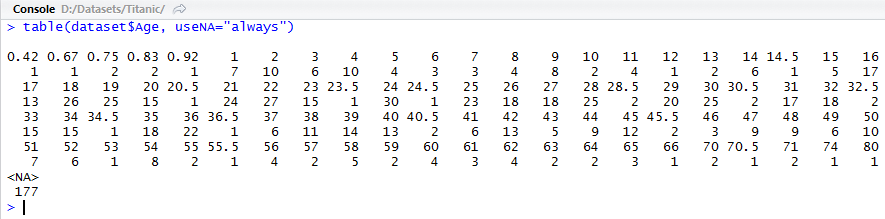
We see 177 missing values (NA's). We will fill them with mean value of Age as a straight forward solution. The commands below store TRUE/FALSE values in a vector bad by checking whether the value of age is available for each record or not, then stores the middle value of age where it is missing and plots the bar graph of age afterwards.

> bad <- is.na(dataset$Age)
> dataset$Age[bad] <- median(dataset$Age, na.rm=TRUE)
> plot(table(dataset$Age))

We now have age with no missing values. In order to simplify our decision rules, we need to change this continuous attribute into discrete valued attribute.

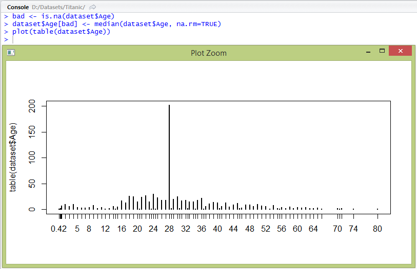
Let's discretize this field into infant, child, teenager, adult and old.

> dataset$AgeGroup <- 'old'
> dataset$AgeGroup[dataset$Age < 2] <- 'infant'
> dataset$AgeGroup[dataset$Age >= 2 & dataset$Age < 13] <- 'child'
> dataset$AgeGroup[dataset$Age >= 13 & dataset$Age < 20] <- 'teenager'
> dataset$AgeGroup[dataset$Age >= 20 & dataset$Age < 40] <- 'young'
> dataset$AgeGroup[dataset$Age >= 40] <- 'old'

> table(dataset$Survived, dataset$AgeGroup)/nrow(dataset)

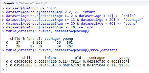
The above distribution tells us that survival rate of infants is very high; children have about half the chance of survival; teenagers and young people have lower and finally, the old have the least survival ratio.

Let's rebuild our model. This time, if a passenger is male, then we make decision on the basis of age variable.

> testset$AgeGroup <- 'old'
> testset$AgeGroup[testset$Age < 2] <- 'infant'
> testset$AgeGroup[testset$Age >= 2 & testset$Age < 13] <- 'child'
> testset$AgeGroup[testset$Age >= 13 & testset$Age < 20] <- 'teenager'
> testset$AgeGroup[testset$Age >= 20 & testset$Age < 40] <- 'young'
> testset$AgeGroup[testset$Age >= 40] <- 'old'
> testset$Survived <- 0
> testset$Survived[testset$Sex == 'female'] <- 1
> male <- testset$Sex == 'male'
> testset$Survived[male & (testset$AgeGroup == 'infant' | testset$AgeGroup == 'child')] <- 1
> submit <- data.frame(PassengerId=testset$PassengerId, Survived=testset$Survived)

> write.csv(submit, file="femailes_and_children_survive.csv", row.names=FALSE)

Let's check what does Kaggle say about our new model.

As seen, our score bumped to 77%. This may not come to you as a very impressive score, but this is not where we are going to stop.

At this point, you must be wondering how complex our code becomes once we start adding more and more attributes. Thumbs up if you wondered this. This is where we make use of smart machine learning algorithms for classification.

Classification Algorithms

We can think of predictive analysis as a case of classification, where we are classifying entities based on some prior information about the domain. Machine learning is a branch of theoretical computing that deals with supervised classification. Supervised in a sense that we first tell the algorithm some information about the data, which the algorithm takes further decisions on the basis of.

Decision tree is among the simple examples of classification where we construct a tree of rules based on probability of occurrences of various events. For example, we earlier made a general rule:

If Sex is female then Survive, otherwise if AgeGroup is infant or child then Survive, otherwise Not Survive.

There is a variety of decision tree algorithms that can be used in R out of the box to create such decision trees automatically. Let's try one...

Recursive partitioning is an implementation of decision trees in rpart package in R, used to for predicting classification trees.

You'll have to first install two packages for rpart and to plot its tree:

> install.packages(c("rpart","rpart.plot"))
> library(rpart)
> library(rpart.plot)
> rpart_fit <- rpart(formula=Survived ~ Sex + Age, data=dataset, method="class")

> prp(rpart_fit, type=1, extra=100, box.col=c("pink", "palegreen3")[rpart_fit$frame$yval])

Here, the rpart() function analyzes the data and gives a model fitting to the data over the given formula. The formula states that the target variable is Survived and decision tree is to be constructed using Sex and Age attributes.

The prp() function plots the learnt tree. This is how it looks like:

The decision tree describes that there are 35% chance of survival when Sex is not male; when Sex is male and AgeGroup is among old, teenager and young, then chances of survival is 4% only.

We will now predict the Survival values using this model. We pass the rpart_fit - the tree learnt, testset and the type of target variable to predict() function, i.e. class.

> testset$Survived <- predict(rpart_fit, testset, type="class")

> submit <- data.frame(PassengerId=testset$PassengerId, Survived=testset$Survived)

> write.csv(submit, file="rpart_sex_agegroup.csv", row.names=FALSE)

The results from Kaggle did not show any improvement from previous results, but we now have a way to add more attributes without having to code complex rules.

Let us now add more attributes to the formula in rpart and see what develops.

> rpart_fit <- rpart(formula=Survived ~ Sex + AgeGroup + Pclass + Embarked, data=dataset, method="class")

> prp(rpart_fit, type=1, extra=100, box.col=c("pink", "palegreen3")[rpart_fit$frame$yval], cex=0.6)

As observed, the decision tree is quite complex after adding only two more attributes to the formula. Imaging writing code for this :-)

Proceed to submitting results on Kaggle.

> testset$Survived <- predict(rpart_fit, testset, type="class")

> submit <- data.frame(PassengerId=testset$PassengerId, Survived=testset$Survived)

> write.csv(submit, file="rpart_more_attr.csv", row.names=FALSE)

This bumped our score to 78.947% and also brings us to 706th rank on the competition.

Let's now attempt to add all of the attributes. But we first need to clean them, right?! Yes, in next part, we will do so.